This is the second post in the series “The Three Deadly Threats to a Clinical Trial - Dare to Risk It?”. For the first part - The Introduction, follow this link .
Even a perfectly conducted clinical trial can end up answering the wrong question if the research objective is misaligned with the statistical hypothesis. It is possible to obtain a technically and factually correct answer to a question that is different from the one asked. As ridiculous as this may sound, it does not happen infrequently. Different perspectives, created by different combinations of endpoint definitions, different moments of observation (or measurement), using different measures to summarize endpoints, and other factors can make the research question inadvertently assigned to a hypothesis that does not accurately represent it.
A clinical trial is conducted to test a specific research question about the treatment being investigated. This defines the objective of the study. The idea seems relatively simple:
Surprisingly, it is relatively easy to conduct an analysis providing answers that are not necessarily in line with the researchers’ intentions. In other words, it is possible to obtain both technically valid and factually correct answer to a question that does not align well with the researcher’s objective, or simply that was never asked.
As absurd as this may sound, it does not happen infrequently and is truly difficult to address, but why (what?) causes it? Let us have a look at the figure below: there can be multiple valid perspectives from which we can look at the truth. Each can be equally correct, yet reveal only part of it, and thus, tell different stories. It is possible to obtain different, though correct, characteristics of the phenomenon investigated. It may potentially lead to different and even inconsistent conclusions, especially if some perspectives are also distorted by unmanaged, often unknown (or unanticipated), factors.
Researchers may then either combine multiple perspectives to not overlook important aspects, or stick to just one, well-grounded in the available domain knowledge.
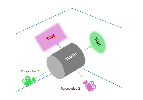
Figure 1: two true reflexes of the unobserved truth - different shapes
Not only the “shape” can vary, but also the observed magnitudes of the effect size, as shown in the next figure. This explains why statisticians are so strict about the evaluated hypotheses and warn against “juggling” with statistical tests (e.g. when assumptions are not met). While a hypothesis expressed in one way may be linked with a large, clinically meaningful effect, different definitions may yield little or no effect.
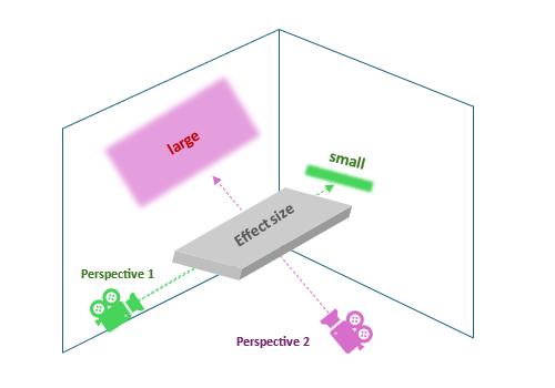
Figure 2: two true reflexes of the unobserved truth - different sizes
But what makes all these different perspectives? Well, a variety of reasons can shape them:
These challenges alone or mixed can reshape the conceptual framework and thus the way linking the observed reality with the phenomena we explore. Let us now briefly explore selected factors.
Some endpoints align with the original question better than others, depending on what aspect of the patient’s condition we are aiming to impact and – fundamentally – how we conceptualize the disease process.
Different parameters can be assessed, both subjective like patient-reported outcomes (e.g. via questionnaires) and objective, such as biochemical markers through laboratory examinations of blood, urine, and other biological materials. A lot of parameters can be collected, related to one specific issue or multiple parts of the biochemical puzzle (non-specific markers).
Consider a hypothetical oncology study of patients with severe anaemia induced by radiotherapy and/or chemotherapy. Such anaemia can cause severe fatigue and significantly reduce the daily quality of life of patients, lead to increased disability, significantly limit the range of daily activities, and even cause depression leading to therapy discontinuation. Relief for patients and improvement of their daily quality of life in this regard is therefore an essential part of supportive oncology care.
Anaemia can be treated in several ways, depending on its level, including supplementation (iron, folic acid, B12 vitamin, etc.) and nutrition support, erythropoiesis (the process that produces red blood cells – erythrocytes) stimulating agents, and ad-hoc blood transfusions, giving immediate relief though not curing the problem itself.
Now, how the progression and recovery are monitored depends on the causes as well as the treatment used to approach the deficits. Haemoglobin concentration is often the first-line parameter to be tracked, as it is the most downstream, clinically visible indicator of anaemia, with immediate clinical guidelines (e.g. for transfusion). But also, the iron metabolism is often of interest, including the level of serum iron, serum ferritin (a protein storing iron), saturation of transferrin (delivers iron to erythroblasts, making it available for erythropoiesis), and the total iron-binding capacity (TIBC). This gives more insight into the anaemia especially if iron levels improve, and yet haemoglobin does not increase.
This story shows that the choice of the target parameter that we shall monitor will be of fundamental importance for our assessment of the effectiveness of the therapy, especially if the relationships between them are complex, non-linear, and delayed.
For this very reason, composite endpoints may be a better choice, allowing for a broader perspective. Only let us not forget that compound endpoints may fail if just one of their components fails. For this reason, we should use components of comparable importance.
In another scenario, we may be interested in counting events reflecting the patient’s condition or measuring the time from the baseline to their occurrence. How such events are defined will fundamentally affect our perception of the situation and decisions made based on that. For example, consider a question like “Does the treatment help patients live better” or “-longer?”. In cardiology and oncology, such questions are often addressed through the survival analysis assessing the time to some – usually unfavourable – event. There are numerous commonly used “time-to-“ definitions, such as Overall Survival (OS), Progression-Free Survival (PFS), Time To Progression (TTP), Disease-Free Survival (DFS), Event-Free Survival (EFS), Time To Treatment Failure (TTTF), Time To Next Treatment (TTNT), Time To Response (TTR) and Duration Of Response, Time To First Recurrence (or Remission), to name a few. Also, the “response” may be defined in a variety of ways. In oncology it can be the “complete response”, “partial response”, “stable disease”, or “progression” (according to the Response Evaluation Criteria In Solid Tumours - RECIST).
Curious readers may find this paper: Delgado A, Guddati AK. Clinical endpoints in oncology - a primer .
And also here the situation can be complicated. For instance, the Progression-Free Survival (PFS) endpoint is often preferred over the “gold standard” – Overall Survival (OS) because of shorter follow-up, leading to reduced costs and faster-making decisions. But the PFS may poorly correlate with OS in certain situations!

For example, the investigated treatment might delay disease progression (improving PFS) but not extend the overall lifespan due to its toxicity (this can happen in oncology). Or, if after the disease progression patients receive highly effective treatments, this can significantly extend the OS, diminishing this way the impact of the evaluated therapy (PFS « OS). Not only that! In case of aggressive tumours OS can be greatly shortened despite benefits in the PFS. Not to mention non-cancer mortality (from co-morbidities), and other reasons further de-correlating the two endpoints.
By the way, you might find these articles:
- Booth CM, Eisenhauer EA, Gyawali B, Tannock IF. Progression-Free Survival Should Not Be Used as a Primary End Point for Registration of Anticancer Drugs
- Amir E, Seruga B, Kwong R, Tannock IF, Ocaña A. Poor Correlation between Progression-free and Overall Survival in Modern Clinical Trials: Are composite endpoints the answer?
- Pasalic D, McGinnis GJ, Fuller CD, Grossberg AJ, Verma V, Mainwaring W, Miller AB, Lin TA, Jethanandani A, Espinoza AF, Diefenhardt M, Das P, Subbiah V, Subbiah IM, Jagsi R, Garden AS, Fokas E, Rödel C, Thomas CR Jr, Minsky BD, Ludmir EB. Progression-Free Survival is a Suboptimal Predictor for Overall Survival Among Metastatic Solid Tumor Clinical Trials
If we add topics like competing risks, presence of terminal events, recurrences, and treatment switches, answering our seemingly simple question: “Does the treatment make patients live longer or better?” becomes even more challenging! Two independent teams can obtain contradictory results for the same treatment, disease, and condition simply by using a slightly different endpoint.
And we did not even start talking about:
All of this information is part of the definition of the study endpoints, and each element can significantly affect endpoint properties and actual meaning.
Once the endpoint is defined, it is time to select the measure to summarize it and make inferences about it.
…it can be, for instance, arithmetic mean, geometric mean, median, or pseudo-median, expressed in the natural units (e.g. mg/dL, IU/L, mmol/L). For symmetric, unimodal distributions (a special case of which is the theoretical Gaussian “normal” distribution) medians and arithmetic means follow each other closely. Ideally, for the theoretical normal distribution – they are equal. As skewness increases, they diverge, as the median is less affected by extreme observations. By the way, this is my routine simple method to assess if asymmetry caused differences too big to be accepted by me. If not, I can safely use the arithmetic mean. One may also use more sophisticated measures such as Fisher’s moment coefficient or quantile-based skewness coefficients.
But the median can also be tricky – just by its definition it is sensitive to the frequency of observations in the middle and can be even affected just by… a single observation! If we analyse data with a big magnitude step in the middle of the sorted measurements (it can happen e.g. in studies on dose reduction), for example {0, 0, 0, 1, 1.5, 10, 60, 65, 76, 89, 90}, then just single observation more from either side can change the value of median greatly. In the given example 10 can turn into 1.5 or 60, respectively. So, both mean and median can be affected just by a single observation, only the mechanism differs.
But this is not all! They have different properties. The mean difference is equal to the difference of means, so the same nominator is shared across the statistical tests for paired and unpaired data. But this does not hold for medians! Median differences (used for paired data) can differ greatly from differences in medians (used for unpaired data) and even have opposite signs.
An interesting case, where mean and median may not be the best measures of central tendency, is multimodal distributions, especially bimodal ones (with two “peaks”), reflecting locally concentrated observations. In case of such distributions it may happen that both mean and median point to the… least probable observation rather than the most common one - look at the figure below.
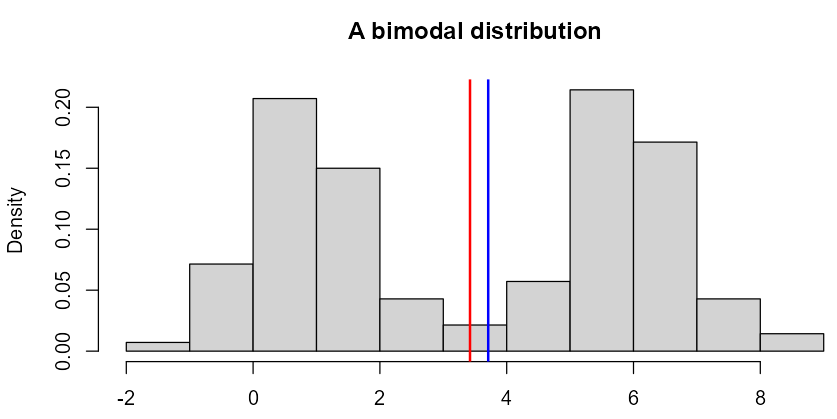
Figure 3: ‘Twin Peaks…’
Bi-modally distributed data usually come from mixtures of individuals with different characteristics. Often such sub-distributions can be separated according to some “discriminating” factors, such as sex, age group, treatment and treatment arm, type and stage of some disease (e.g. cancer), taking certain medications, drinking alcohol, etc.
For example, in oncology certain types of cancer follow a bimodal pattern, including: acute lymphoblastic leukaemia, osteosarcoma, Kaposi Sarcoma, Hodgkin’s lymphoma, germ cell tumours, and breast cancer (Desai S, Guddati AK. Bimodal Age Distribution in Cancer Incidence ). Other interesting examples can also be found in:
Sometimes, however, such factors remain unknown, which prevents us from separating such subgroups. Then, whatever we observe – bi-modality or asymmetries, have to be treated as a whole. Especially in the case of skewed distributions it is important to distinguish the source of asymmetry caused by the statistical “nature” of the data, such as counts, time-to-event data, limited data or caused by multiplicatively-acting processes (e.g. cascading biochemical reactions, driven by hormones and enzymes; common in pharmacokinetic analyses) from skewness caused by mixed subpopulations. Such subpopulations locally can be perfectly approximated by a Gaussian distribution, but combined they can appear extremely skewed (right- or left-sided), which often leads to completely unnecessary and scientifically unjustified transformations of the data (e.g. logarithmic transformation). If you are interested in the same topic, check out our other post: On the ubiquity of skewness in nature: challenging the cult of the prevalent normal distribution .
By the way, such (non-linear) transformations can modify the perspective and therefore alter the answered questions as well!
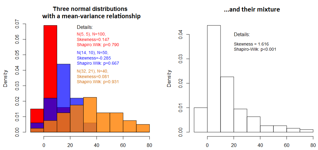
Figure 4: Example of how a mixture of distributions can cause skewness
In the case of more difficult distributions, we may need more than just single-number measures. We can use the “Tukey’s Five”: minimum, Q1, Q2 (median), Q3, and maximum, supported also by the arithmetic mean. In such cases, comparing just means or medians may be pointless, with the need for other approaches.
It is also not uncommon that the comparison expressed in terms of means may lead to different even opposite conclusions than comparing medians. This is why statisticians are so unhappy to “juggle” statistical tests and switch to non-parametric, rank-based, or quantile-based ones when the parametric assumptions are not met. Luckily distribution-free methods preserve the original null hypothesis, such as permutation Welch t-test, general equation estimation (GEE), and some modification of the ordinal logistic regression applied to numerical data (yes, you read well!). I hope to cover this topic in a separate series of blog posts [Test your hypotheses like a pro!].
Sometimes we are interested in more “exotic” things like “stochastic superiority”, that is, the probability that one sample consistently dominates over the other. In other words, this means that for a pair of observations sampled from both compared samples (A, B), the probability that P(A < B) is larger than 50%. The idea of stochastic superiority can be visualized in the figure below: there are two variables (endpoints), A and B. We connect all pairs of observations from both groups (b1 with every ai, b2 with every ai, etc), then, for each pair, we determine their relationship (B>A - green, B ≤ A - red) and count all pairs where B > A. Dividing this count by the number of all pairs gives the % of superiority. Indeed, in the figure, the number of red-marked pairs is much smaller than the green ones.
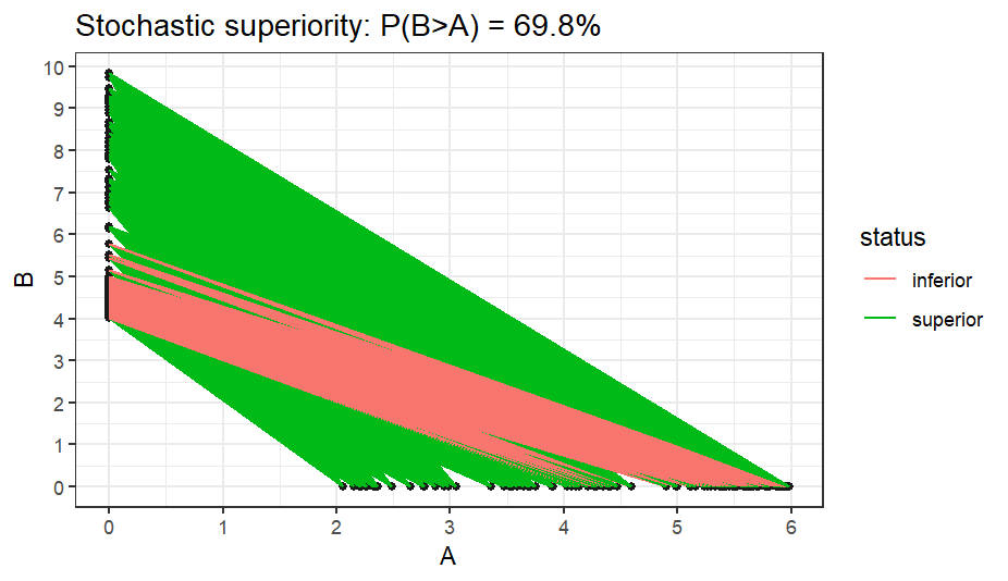
Figure 5: Illustration of the idea of stochastic superiority (dominance)
Stochastic superiority is a very general property and is closely related to ranking the raw data. The ranking is a monotonous transformation that ignores magnitudes, so only the precedence of observations is retained.
Analysis of raw means is now replaced by analysis of mean ranks. But this does not easily translate into (non-) equality of raw means or medians. It may happen that stochastic superiority is achieved for equal arithmetic means or medians, due to differences in variances, skewness, modes and and other elements of the distribution shape. And the contrary holds too: means or medians can differ noticeably, while stochastic superiority will not be claimed.

Figure 6: Stochastic superiority can be reflected by many things
By the way, this is precisely what rank-based non-parametric methods like the Mann-Whitney (-Wilcoxon) or Kruskal-Wallis methods deal with. In the example below superiority is claimed for equal means or medians. For means I used the Welch-Satterthwaite version of the t-test and compared it against the Mann-Whitney test. For medians, I used the Mood’s-Brown test (I could also use quantile regression) against the Mann-Whitney test. While the “dedicated” tests properly reported no difference (p-value = 1), Mann-Whitney, in both cases reported a p-value <0.001.

Figure 7: Stochastic superiority may be claimed despite equal means…
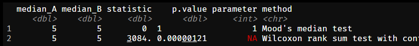
Figure 8: …or medians!
We will get back to this topic a bit later, when discussing statistical misconceptions about non-parametric statistical tests used commonly to compare numerical outcomes.
…such as clinical successes, are usually summarized with proportions (also called “risks”) and their differences (RD; expressed in percentage points), risk ratios (RR), and odds ratios (OR). Time-to-event outcomes can be assessed through survival times or hazard ratios (HR). And also here there can be problems. For instance, odds ratios are called “non-collapsible measures”, which means that these ratios calculated across sub-groups may not be aligned with the total ratio (unlike means and the absolute risk reduction). This happens because odds are a *non-linear transformation of probabilities. Testing differences about proportions can be done on either the log-odds scale or the probability scale, which – for probabilities outside the (approximately) linear region (i.e. between 0.15 and 0.85) can diverge from each other.
… can be summarized with hazard rates, restricted mean survival time (RMST), survival probability at a fixed moment, quantile of the survival time (if achievable), and the change in time-to-event (e.g. via parametric Accelerated Failure Time; AFT models). All are valid, and all pose certain challenges. Survival quantiles may not be achievable. Hazard ratios are best interpretable at proportional hazards, though it’s not critical, this discussion exceeds this post, and non-crossing survival curves – though there exist tests and methods to handle these cases. RMST needs no assumptions and can be calculated also in the presence of crossing curves, which is a bit more complex to interpret. Time-to-event obtained from the AFT model requires the assumption about the distribution used to model the events’ times. Also, a similar measure is the fixed-timepoint survival probability (SP).
While, for instance, the survival probability is about the likelihood of surviving past a point, the RMST is about the average duration of survival within a defined period. This perfectly shows how different perspectives can be assessed through just a single analysis! One says, “What percentage of patients survive to a specific time?”, the other – “On average, how long do patients survive up to a certain time?”.
In the presence of competing risks, we may also be interested in the cumulative incidence function (CIF) and cumulative probability of some events. Recurrent events combined with terminal events may complicate things even more! There is also an ongoing debate on whether to use the competing risks or the cause-specific hazards (censoring the competing risks) for the causal analysis.
As we can expect, each decision, and each measure selection will answer a different question. In some scenarios these questions will be consistent, in others – they will conceptually diverge.
One of the biggest challenges with statistical tests is understanding what they actually test, i.e. their null and alternative hypothesis. Too many misconceptions are present even in peer-reviewed papers and textbooks, which are then spread over and over by their readers. Practitioners may be then misguided and interpret the results of certain tests incorrectly.
One of my favourite topics is “What do Mann-Whitney (-Wilcoxon) and Kruskal-Wallis tests assess?”. Many researchers and some statisticians may quickly respond: “They assess the equality of medians!”. And they will be wrong in general.
Let us have a look at the following figure. It shows one of my examples instantly disproving that Mann-Whitney (-Wilcoxon), its improved “brother” Brunner-Munzel, and Kruskal-Wallis tests assess the equality of medians. They do not, unless a strong and rare condition is met: compared samples must be “IID”, meaning independent-and-identically-distributed. The “identically distributed” here means: same variance (dispersion in data) and shape of the distribution (can be skewed, but both in the same way). Only then, the only that left to vary is the “shift in location”, meaning the difference in medians. But this is a theoretical condition and will never occur in practice, therefore this test can compare medians (under the given condition) only approximately.
This problem is known as the non-parametric generalized Behrens-Fisher problem, i.e. to compare locations when dispersions and other properties of the distributions vary.
Here variances are comparable, medians are exactly equal, and yet the p-values are very small at just moderate sample sizes. When we look at how these boxplots are placed concerning each other, we can see that for each pair one dominates over the other. This is exactly the stochastic superiority case, that we discussed earlier!
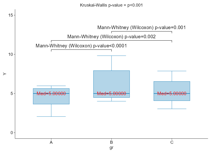
Figure 9: Mann-Whitney and Kruskal-Wallis do NOT compare medians in general!
Let me reuse the example I showed above. Now, the variables are put in front of each other and additional measures are displayed: difference of medians, median difference, 2-sample pseudo-median, Mann-Whitney p-value intentionally showing so many decimal digits, and the result of quantile regression-based test for medians. Below I show the empirical cumulative distribution functions supported by the Kolmogorov-Smirnov test.
Look at the result of the Mann-Whitney test: superiority is claimed despite equal medians, and it agrees with the test of empirical cumulative distribution functions.
Figure 10: Stochastic superiority under equal medians
But look, what happened in the second example? Now the superiority cannot be claimed (regardless of sample size!), despite different medians, means, and the whole distributions! You can also notice, how the median difference disagrees with the difference in medians, even the signs are different.
How did I find such a configuration of data? Well, if you understand the idea of superiority, you can prepare the data accordingly. I exaggerated the pattern a bit to make it better visible. In real cases, the data will be much more messy, and you may be surprised by the result of rank-based methods!
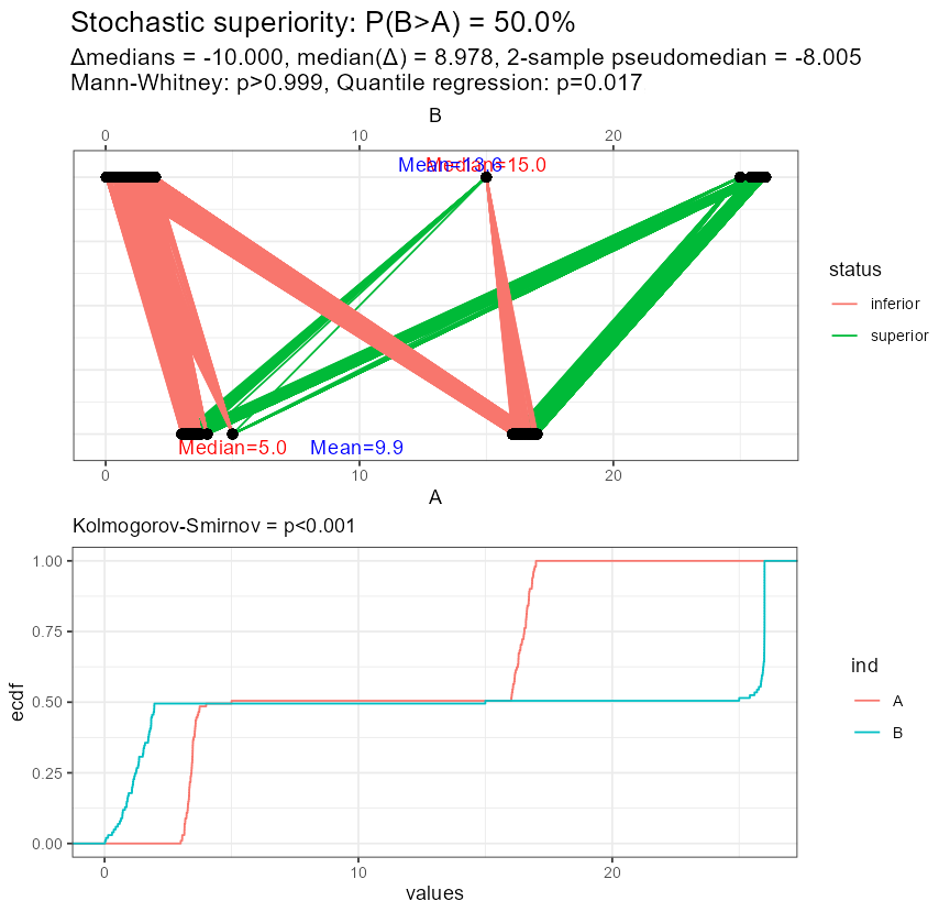
Figure 11: Stochastic equivalence under different medians
It is worth noting that the original papers by Wilcoxon (" Individual Comparisons by Ranking Methods "free PDF) and Mann-Whitney (" On a Test of Whether one of Two Random Variables is Stochastically Larger than the Other "free PDF) do not refer to medians.
On this topic, I strongly recommend these two books:

Figure 13: Recommended books about the rank-based tests
Not only you will learn about modern replacements for Kruskal-Wallis, allowing you to test multiple factors and their interactions, repeated observations, such as ANOVA-Type Statistic (ATS) and Wald-Type Statistic (WTS), but they also explain the above phenomena on the mathematical ground. For example, we can learn that:
Source: E. Brunner, A. C. Bathke, F. Konietschke , “Rank and Pseudo-Rank Procedures for Independent Observations in Factorial Designs using R and SAS”
These books should be available at Google Books (that’s how I took these screenshots), so you can browse them before buying.
Now it should be clear that switching from parametric methods to non-parametric methods (e.g. rank-based, quantile-based) will inevitably switch your original null hypothesis from, say, comparing means, to something else, e.g. comparing medians or mean ranks = assessing stochastic superiority. Depending on the distribution of your data, these hypotheses may be consistent or not. In other words, by changing the statistical method you change the answered question!
The good news is that there exist distribution-free methods that preserve the null hypothesis. I am going to describe them in a separate post [Test your hypotheses like a pro!]. You should always plot your data and examine it before blindly interpreting the results of non-parametric tests!
Such change of analytical method based on the result of the assessment of statistical assumptions pertains to other areas too, for example, survival analysis, that we already discussed. In particular, if due to strongly violated proportionality of hazards you switch from Cox regression to Accelerated Failure Time (AFT) parametric survival model, from the long-rank test to weighted log-rank (e.g. Peto-Peto, Gehan-Breslow, Tarone-Ware), from log-rank to Max-Combo and the whole Flemington-Harrington weighted log-rank family, from hazard ratio to RMST and other measures – you look at the data from a different perspective and potentially tell a different story.
There exist many other statistical misconceptions, such as when to test main effects in the presence of interactions (yes, this IS possible, despite a popular claim that it’s “always disallowed”, but you must make sure it’s not a dis-ordinal interaction and do some additional checking).
Let us recall the already mentioned anaemia case. Patients are treated with erythropoiesis stimulants, hoping to increase the level of haemoglobin. If we ignore the type of cancer and its stage in the analysis, we may observe that the higher the administered dose, the higher the mortality and the poorer the response! One explanation is that patients with certain kinds of cancer (e.g. colorectal) may experience occult bleeding. In addition, those already in palliative care may develop much worse organism response to treatment, despite the highest doses of erythropoiesis stimulants administered to improve their daily quality of life. Also, patients in the terminal stage will eventually die, increasing the mortality rate. At the same time, even a small increase in haemoglobin level can be a relief, even despite possible side reactions. For patients with less advanced cancer or in remission, significantly smaller doses are sufficient to cause good responses, and the mortality rate is much smaller. Effectively, it turns out that the treatment works well, but the omitted confounding factor “cancer type and stage” distorts the picture of the situation, creating the false impression that the therapy is futile and toxic!
Specialists in the causal analysis will recognize a typical problem, where to correctly estimate the total effect of some exposure (here: stimulants of erythropoiesis) on some outcome (here: fatigue caused by anaemia, optionally mortality – for safety analysis) one has to account for a confounder (here: the type and stage of cancer) to avoid spurious relationships. A Directed Acyclic Graph (DAG) can be found in the following figure. This kind of confounder will “act” continuously after the randomization and change the dynamics of its impact over time (a time-dependent factor).
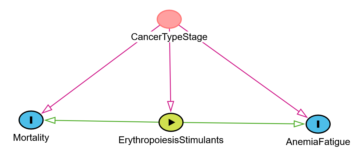
Figure 14 A Directed Acyclic Graph for the described example
The combination of an endpoint, a measure used to summarize it, a time point, along with some logical operators and additional information (such as the margin of non-inferiority), defines a statistical hypothesis into which researchers translate the goals of their research. By choosing different “ingredients,” one effectively creates a different hypothesis. In this way, the research question can be inadvertently assigned to a hypothesis that does not accurately represent it. Statistical hypotheses are inseparable from the tests that verify them. The results of statistical methods can also be misinterpreted (virtually creating a new hypothesis). Diagnostics of the assumptions of parametric methods can lead to the use of alternatives (e.g. non-parametric methods) which may also change the planned hypotheses.
In this way, the chain of “research questions” – “hypotheses” can be broken at many levels, often unconsciously!
Dare to risk it?
To be continued…


I collected for you a few links explaining some topics we have been discussing in this post. Happy reading!
If you’re thinking of your study design audit or rescue action contact us at or discover our other CRO services .
2KMM Sp. z o.o.
ul. Strzelców Bytomskich 3
40-310 Katowice
Polska / Poland


